Customer Analytics with Python – preparing data

In the last part we used a kaggle dataset and prepared a RFM Segmentation to cluster customer transactions. In this part we continue with the data preparation to enable k-means clustering.

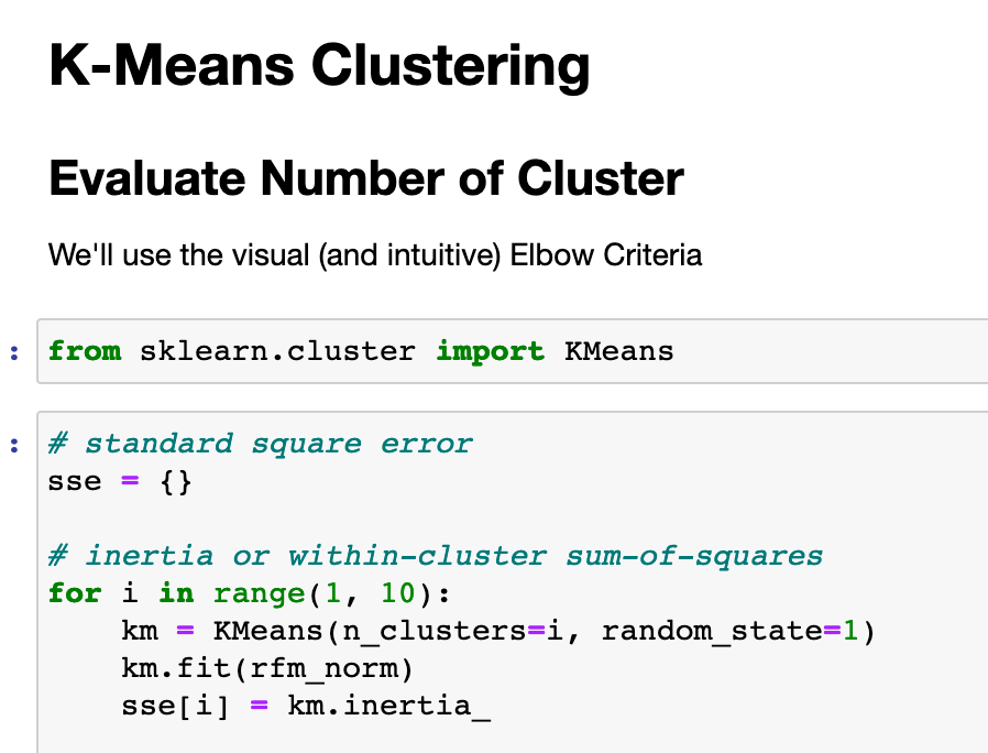
Why k-means and what do we need to do?

K-means clustering is simply fast, there are a tons of tutorials and we can analyze our data more in depth – the world is complex, we should better deal with it!

We need to ensure:

1. a symmetric distribution for our numerical variables (= not skewed!)
2. same average values and same standard deviation

For a better understanding, we’ll do that manually and afterwards we’ll use the sklearn StandardScaler.

Ready, set, go!!

Data preparation for k-means clustering

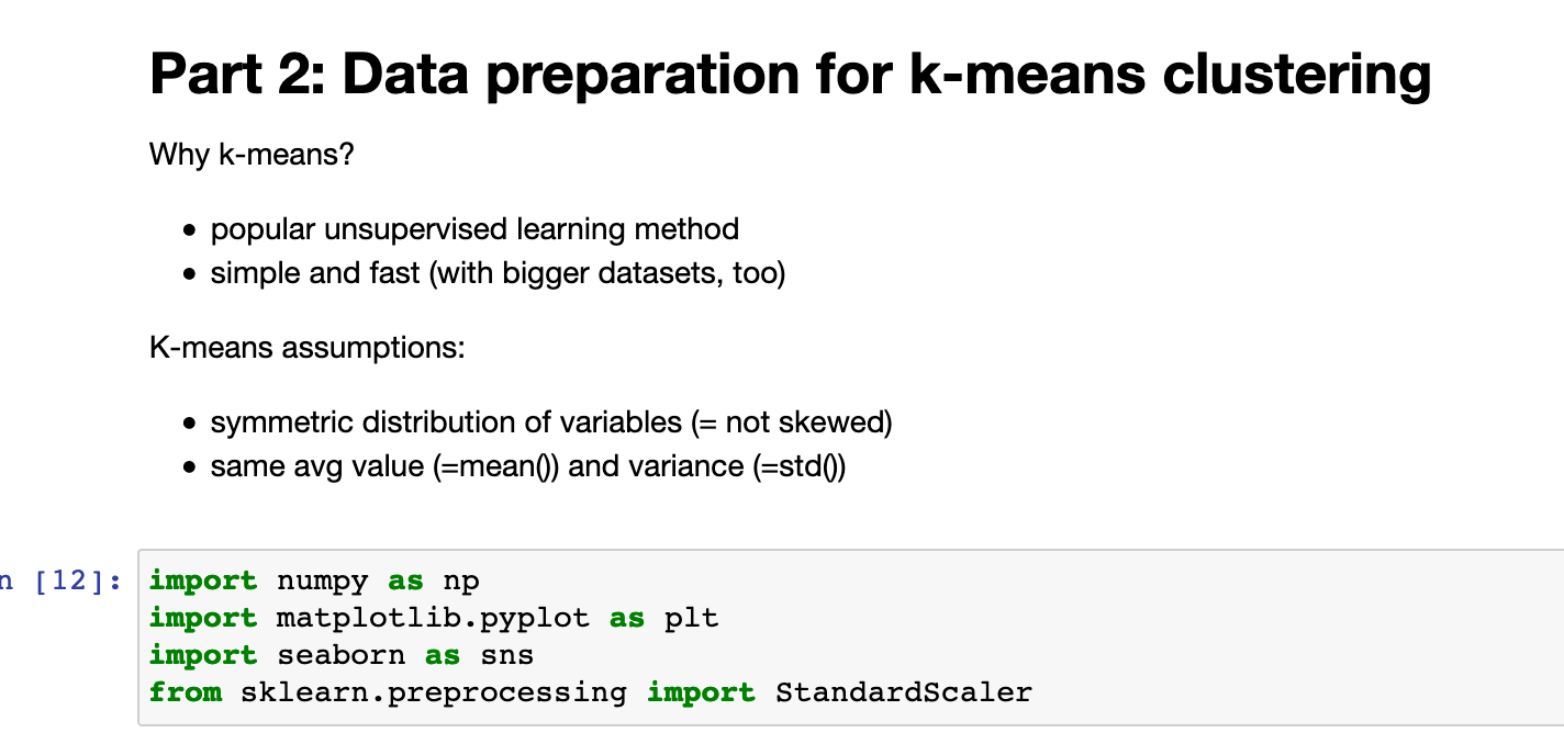
We start by importing the (additionally – see Part 1) necessary stuff and prepare the subset of your Part 1 RFM analysis result.

import numpy as np
import matplotlib.pyplot as plt
import seaborn as sns
from sklearn.preprocessing import StandardScaler

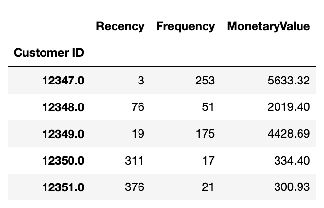
# subset necessary values
rfm_data = rfm[['Recency', 'Frequency', 'MonetaryValue']]
  
# less than 100 rows MonetaryValue < 0
# why do we've this rows? how can a customer have a neg monetary value? -> XMas? Order in 2009 and return in 2010!
rfm_data = rfm_data.loc[rfm_data['MonetaryValue'] > 0]

rfm_data.head()
rfm_data.describe().round(2)

• 

• 

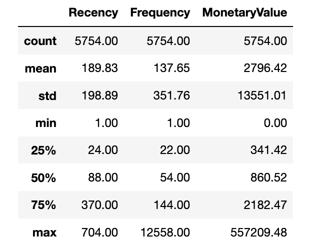
What do we see – how does it look?

# plt.figure defines the size of the plots... feel free
plt.figure(figsize=(15,5))
plt.subplot(1,3,1);sns.distplot(rfm_data['Recency'])
plt.subplot(1,3,2);sns.distplot(rfm_data['Frequency'])
plt.subplot(1,3,3);sns.distplot(rfm_data['MonetaryValue'])
plt.show()

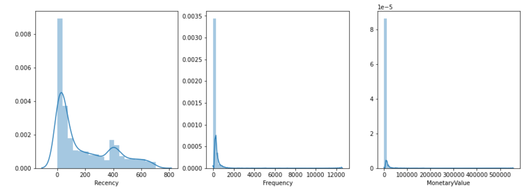
Okay, we’ve:

• unequal mean and std for our values
• right-skewed distribution
• we already dropped negativ values and can perform log() to „fix“ the skew

As an example – the Frequency value

freq_log = np.log(rfm_data['Frequency'])

sns.distplot(freq_log)
plt.show()

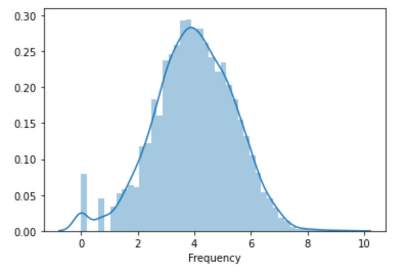
We can perform the log() to the dataframe by

rfm_log = np.log(rfm_data)
rfm_log.describe().round(2)

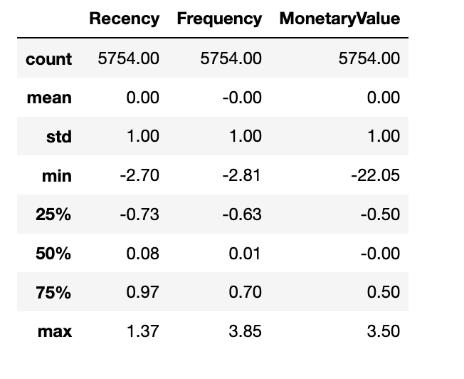
and standardize and scale by

# standardize data - data.mean()
# scale data/data.std()

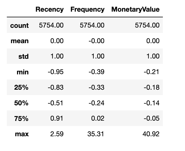
rfm_prep = (rfm_log - rfm_log.mean())/rfm_log.std()
rfm_prep.describe().round(2)

Tipp: round the values! The value won’t be equal in sense of strictly equal.

How to use the sklearn Standard.Scaler()

Instead of doing it manually, we should use sklearn StandardScaler(). Take care of the negative and missing values, to perform a logarithmic transformation of the skewed data and than use the Standard.Scaler. Keep in mind that StandardScaler.transform returns a np.narray and feel free to define a pd.Dataframe out of it.

# log skewed data (before we deleted the <100 rows neg. MonetaryValue)
rfm_log = np.log(rfm_data)

# Normalize
scaler = StandardScaler()
scaler.fit(rfm_data)

# scaler returns a np.narray -> transform to dataframe
rfm_np_norm = scaler.transform(rfm_data)

# rfm_norm is the result and pre processed data for the k-means
rfm_norm = pd.DataFrame(rfm_np_norm, index=rfm_data.index, columns=rfm_data.columns)
rfm_norm.describe().round(2)

Wrap up

We’re done. The effort created with the data preparation, taking care of the zero and negativ values… and than it’s straightforward. Keep in mind that the process is important (zeros -> log() -> standardize&scale!)

Read more – Part 3: Customer Analytics with Python – KMeans Clustering